PYBAMM / WORKED EXAMPLE

Your first battery charge–discharge simulation

Follow one executed Chen2020 example from its input protocol to three readable curves. This is a reference simulation, not measured battery data.

Checking saved status…

Executed 2026-10-20SPM · Chen2020Simulated protocol 22 min

Reproduce this example Code & data

First, look at the result

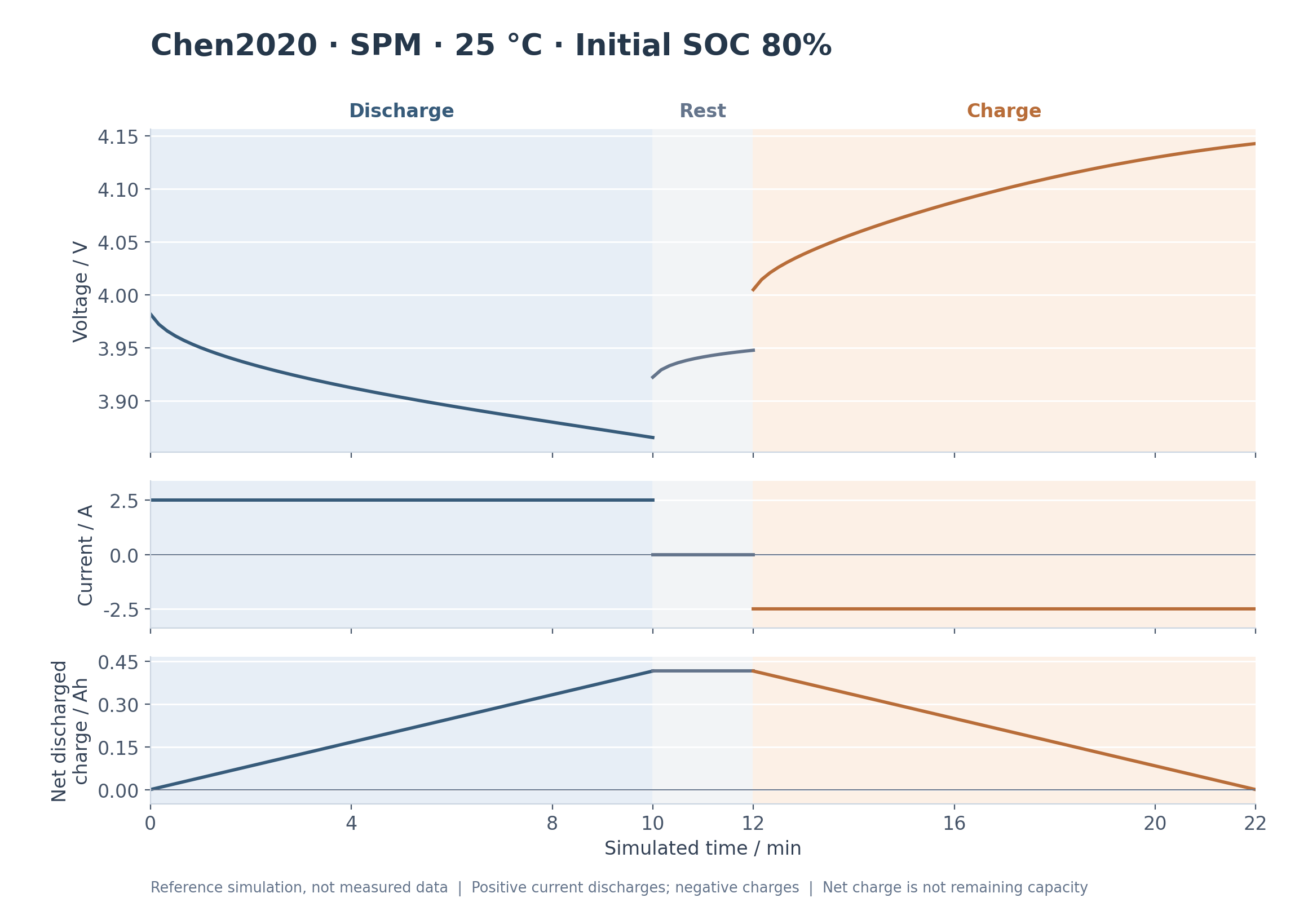
Read the three panels on the same time axis. Positive current is discharge; negative current is charge; zero current is rest.

Executed reference simulation: aligned voltage, current and net discharged charge curves over time. — Generated from this example's CSV: 135 recorded samples over 1,320 simulated seconds. This duration is the modeled protocol, not the computer's running time.
Open full-size figure

Voltage range: 3.8655–4.1429 V
Charge discharged: 0.4167 Ah
Charge charged: 0.4167 Ah
Final net discharged charge: ≈0 Ah

Why does net discharged charge return close to zero?

Net discharged charge is the charge sent out during discharge minus the charge put back during charging. It is not the cell's total capacity. Returning roughly the same charge makes this running total approach zero; it does not mean the battery has no capacity, its SOC returns exactly, or there is no energy loss. It does not establish battery lifetime either.

Understand the inputs

This example uses the single-particle model (SPM) with the Chen2020 parameter set. SPM approximates each electrode with one representative particle; this case does not resolve full electrolyte transport. It is a teaching case, rather than a fit to your own battery.

Initial state of charge: 80%
Temperature: 298.15 K (25 °C)
Nominal capacity: 5 Ah
Sampling period: 10 s

C-rate converts nominal capacity into current. Here, 0.5C × 5 Ah = 2.5 A. The discharge step uses the positive current, and the charge step uses the negative current.

The three finite protocol steps
Step	Simulated time	Current	Start → end voltage
1. Discharge	0–600 s	2.5 A	3.9821 → 3.8655 V
2. Rest	600–720 s	0 A	3.9224 → 3.9478 V
3. Charge	720–1,320 s	-2.5 A	4.005 → 4.1429 V

Each step has a finite duration. The report records why it stopped; this example does not demonstrate voltage-cutoff events or test a hardware operating limit. Keep the supplied protocol unchanged for your first reproduction.

Run it in your own project

Download and extract the example into a new folder. Install Python 3.12 first, then open a terminal in that folder and choose your operating system below.

Create an isolated Python environment and install the locked dependency versions. This installation requires network access.
Run the supplied protocol into a new my-run folder. Make the figures in my-figures so the reference outputs stay intact.
Compare your report and curves with the supplied reference. Runtime and small numerical differences depend on the environment.

The lockfile records this run's Windows / Python 3.12 environment. macOS and Linux need compatible package wheels. If installation fails, inspect the Python version, architecture and error before adapting dependencies; do not change versions blindly. requirements.txt lists the direct dependencies for an informed adaptation; record any differences and repeat the checks.

Windows PowerShell

py -3.12 -m venv .venv
.\.venv\Scripts\python.exe -m pip install -r requirements-lock.txt
.\.venv\Scripts\python.exe simulate_battery.py protocol.json --output my-run
.\.venv\Scripts\python.exe plot_results.py my-run --output my-figures

You can also select and copy the commands manually.

These commands run locally and do not need an AI API key. This page does not run simulations or receive your files. To work through the case with Codex or Claude Code, open this folder as a project and use the installation and first-use requests in the Skill guide.

Open the Skill installation and first-use guide

Check the result, not just the picture

The run compares a baseline calculation with tighter solver tolerances, then with a finer mesh. The report evaluates 101 interpolation points within each corresponding step. The changes below are the largest at those sampled points, not a global error bound or proof of convergence.

Comparison	Largest sampled voltage change
Baseline → tighter solver tolerances	0.001 mV
Tight solver, mesh 20 → 40	2.1686 mV

Largest end-time difference: 0 s. A numerically stable result is not proof that it matches a real battery. The parameters, initial state and measurements would need separate checks.

Which files should I inspect?

curve.csv contains the baseline time series. Compare it with tight-tolerance.csv and refined-mesh.csv. Read report.json for the settings and checks, and parameters.json for parameter provenance. The base Current function [A] parameter is not the actual current for every step: protocol.json sets each step's current. Preserve both files for reproduction.

Execution environment, tolerances and source

Executed on 2026-10-20. This record covers this reference simulation only, not every Skill workflow or a measured-cell validation.

Final net discharged charge, unrounded: 8.534839501805891e-16 Ah

pybamm: 26.9.0.0
pybammsolvers: 0.10.0
numpy: 2.5.4
scipy: 1.18.1
casadi: 3.8.1
matplotlib: 3.10.7
python: 3.12.14
platform: Windows x64
Baseline rtol / atol: 1.000e-6 / 1.000e-8
Tight rtol / atol: 1.000e-8 / 1.000e-10
Skill version: 1.1
Upstream commit: 593377bb048752abb0152deab9fbb1083a6087df
Script SHA-256: 96c9c774860a80f3fddda2fd94d90905e9254b766f191a79e843613ec4da7647
Protocol SHA-256: f769f94f1a9f933d253b3a4a6f51dc661b8af49bf9df52cfdabd81ea185de80e

The PyBaMM library is licensed under BSD-3-Clause. The K-Dense Inc. Skill and simulation helper use MIT; other dependencies retain their own terms. The example preserves the component notices and source credit. Chen2020 is a PyBaMM reference parameter set, and this case uses no measured data.

Keep the complete reproducible example

The bundle contains the simulation and plotting scripts, original protocol, dependency lists, reference CSVs and reports, figures, README, recording script and component licence notices.

Download example code & data · Checking availability…

An account is required. Your download continues after sign-in.

Bundle 1.0.1 · 400,982 bytes
SHA-256: 9088ac565a8984a921ae9b58a9d5f704c69068c039ace1231d6864b0a5767464

A 5–7 minute recording outline

Use the sections above as a recording sequence. This is an outline for presenting the executed example; the downloads include a Chinese script.

0:00–0:35Introduce the reference simulation and what it can answer.
0:35–1:20Read the three protocol steps, initial SOC and temperature.
1:20–2:10Download the example, open a new project and explain the environment.
2:10–3:00Run the commands; show the output folders without promising a fixed runtime.
3:00–4:30Read the voltage/current plots and explain net discharged charge.
4:30–5:40Compare solver tolerances and mesh density; distinguish numerical from experimental checks.
5:40–6:20Show the report, source versions and how to reproduce the case.